Optimal Poker Bankroll Management
1 Introduction
The central question in poker bankroll management is which game to play given a current bankroll. The naive answer — play the game with the highest expected hourly winrate — ignores a key feature of the problem: bankroll is not just a consumption good. It is also a capital good. A larger bankroll unlocks access to higher-stakes games, which offer a higher rate of converting time into money. This means the value of a dollar depends on where it puts you relative to the next move-up threshold.
Because losses are more costly than equal-sized gains — losses delay or foreclose a move up, destroying option value on top of the direct loss — a player with a risk-neutral terminal payoff will behave as if risk-averse in game selection. This risk aversion is not assumed; it is a consequence of the discrete structure of available games.
This document presents two models for deriving optimal game-selection rules. The finite-horizon DP solves the problem by backward induction over a fixed time horizon. The infinite-horizon OBM finds a stationary policy via value iteration, using the Certainty-Equivalent Winrate (CEW) as its convergence criterion and main output. Both are benchmarked against the Kelly criterion; comparing the two is the central result.
2 The Finite-Horizon Model
2.1 Setup
Each period the player holds bankroll \(x\) and selects one of \(N\) games. Transitions follow a Bernoulli stack-off rule: with probability \(p_i = (\sigma_i / B_i)^2\) the player wins or loses a full buyin \(B_i\); otherwise the bankroll shifts by the mean gain \(\mu_i\). A game is only available when \(x \geq B_i + x_{\min}\). The terminal payoff is \(V_T(x) = x\) — no curvature, no risk aversion by assumption.
The model is solved by backward induction from the known terminal value, computing the optimal game at each bankroll level for each period \(t = T-1, \ldots, 0\).
2.2 Game parameters
| Game | Buyin \(B\) | Mean gain \(\mu\) ($/hr) | Std dev \(\sigma\) ($/hr) |
|---|---|---|---|
| Work (outside option) | — | 7 | 0 |
| 1/2 NL | 200 | 12 | 80 |
| 2/5 NL | 500 | 20 | 250 |
Work is a risk-free outside option available at any bankroll. The 1/2 and 2/5 games offer higher expected returns but require sufficient bankroll to cover the buyin.
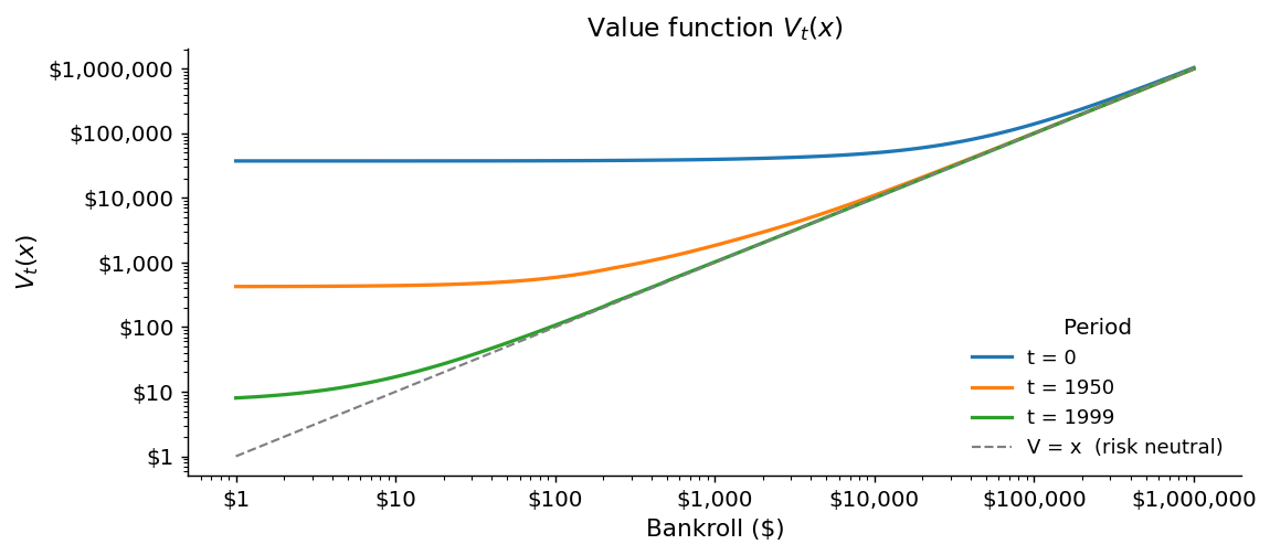
2.3 Optimal policy and value function
The figures below show the optimal game (left) and value function (right) for three periods: \(t = 0\) (far from the horizon), \(t = 1950\) (50 periods remaining), and \(t = 1999\) (final period).
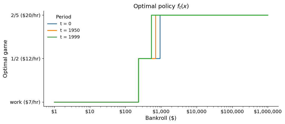
At \(t = 0\), the policy switches from 1/2 to 2/5 at a bankroll of roughly $811–$933. As the horizon shortens, the threshold falls — with fewer periods remaining, there is less time for the option value of higher stakes to compound, so the player moves up sooner. At \(t = 1999\), the player selects the game with the highest raw EV, since no future optionality remains.
2.4 Implied risk aversion
Although the terminal payoff is risk-neutral, the value function is concave in bankroll. The figure below recovers the implied CRRA coefficient \(\eta(x)\) at \(t = 0\) by inverting the local ratio of CRRA utilities at consecutive grid points. The reference line at \(\eta = 1\) marks log utility — the Kelly criterion’s implicit utility function.
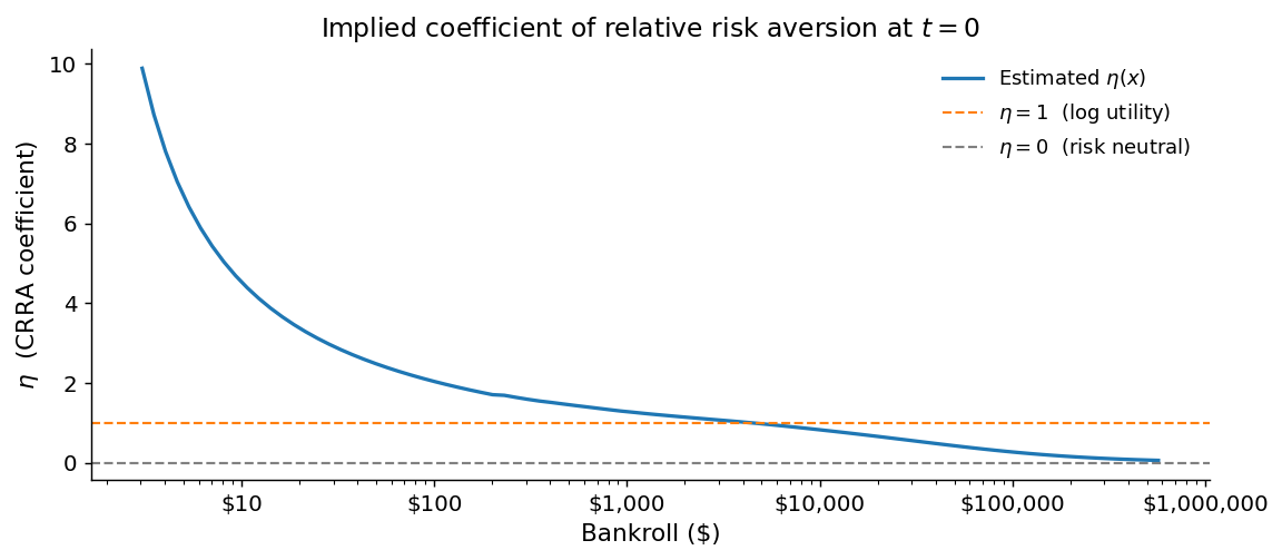
The plot reveals a clean pattern relative to the Kelly benchmark. For bankrolls up to roughly $10,000, the implied \(\eta\) exceeds 1: the discrete option value of the 1/2 game is large relative to current stakes, producing stronger risk aversion than log utility. Above that range, \(\eta\) falls below 1 and continues declining toward zero as no binding move-up threshold remains. Kelly is thus neither uniformly too conservative nor uniformly too aggressive — it underestimates risk aversion at low bankrolls and overestimates it at high ones. The curvature comes entirely from the discrete game structure, not from any preference assumption.
3 The Infinite-Horizon OBM Model
3.1 Setup and the CEW metric
The finite-horizon model requires specifying a time horizon. The infinite-horizon OBM drops this requirement and solves for a stationary policy via value iteration: starting from an initial value function, compute \(E[V(x')]\) for each game, update \(V\), and repeat until convergence.
Convergence is measured using the Certainty-Equivalent Winrate (CEW). The CEW at bankroll \(x\) for game \(n\) is the fixed dollar amount per period that leaves the player indifferent between accepting it and playing game \(n\) under the current value function. It is a bankroll-adjusted winrate: a high-variance game may have low CEW at small bankrolls but high CEW at large ones. The optimal game at any bankroll is the one with the highest CEW.
3.2 Kelly as a benchmark
Kelly (1956) derived the optimal BRM strategy under the assumption that game conditions scale continuously and linearly with bet size — the player can always stake exactly the fraction of bankroll that maximises expected log growth. Under these assumptions, Kelly is genuinely optimal without imposing any exogenous risk aversion; the log-utility behavior emerges from the objective of maximising long-run bankroll growth. In that setting, the implied CRRA coefficient is exactly 1 everywhere.
Chen & Ankenman (2006) use Kelly as a benchmark for optimal BRM in poker, but acknowledge that the continuous scaling assumption does not match the discrete structure of real game selection: a player cannot stake an arbitrary fraction of their bankroll, only choose among a fixed menu of games with fixed buyin sizes. They interpret Kelly as an approximation to the true optimal policy; alternatively, it can be understood as imposing log utility as an exogenous preference rather than deriving it from first principles.
The OBM model derives the actual optimal policy under discrete game choice, without assuming any utility function. Risk aversion emerges endogenously from the option value structure of the game menu. Kelly is computed here as the one-shot benchmark — setting the value function to \(\log(x)\) and solving in closed form without iteration — and the gap between Kelly and OBM quantifies what recursive optionality pricing adds.
3.3 Game parameters
| Game | Buyin \(B\) | Winrate \(w\) ($/hr) | Std dev \(\sigma\) ($/hr) | Min viable bankroll |
|---|---|---|---|---|
| Work | — | 5 | 0 | — |
| 1/2 NL | 100 | 10 | 100 | $300 |
| 2/5 NL | 200 | 15 | 200 | $600 |
| 5/10 NL | 500 | 20 | 500 | $1,500 |
A game is available only when the bankroll exceeds twice the buyin and three standard deviations, below which the normal approximation to the session outcome breaks down.
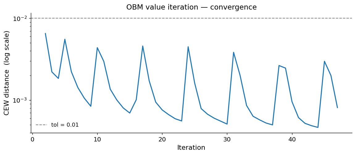
3.4 Convergence
Value iteration converges in 47 iterations, taking under a second. The plot below shows the max relative change in CEW per iteration, starting from iteration 2.
3.5 CEW curves
The figures below show the per-game CEW under OBM (left) and Kelly (right). Dotted horizontals mark true hourly EV; dashed verticals mark move-up thresholds.
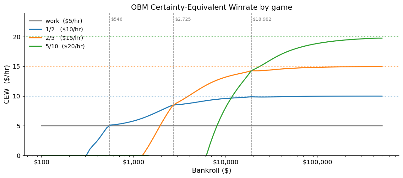
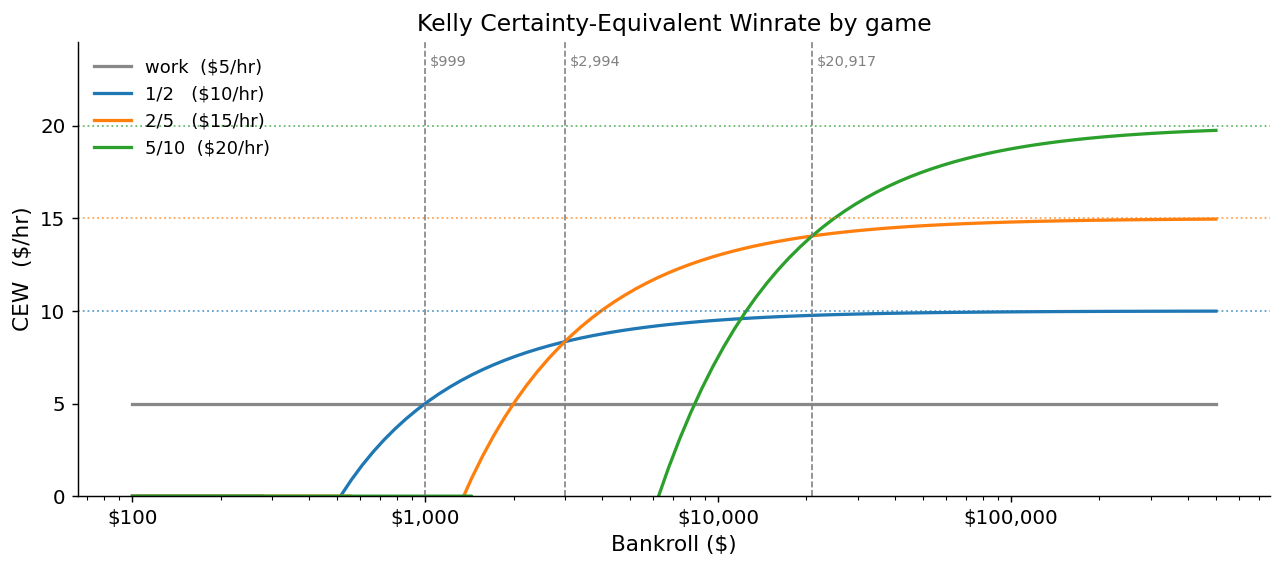
Both models produce qualitatively similar CEW curves with well-defined crossings that define move-up thresholds. OBM CEW rises more steeply at low bankrolls because the recursive model prices near-term option value more aggressively than Kelly.
3.6 OBM vs Kelly: interpretation
The comparison between OBM and Kelly is the central result of this analysis.
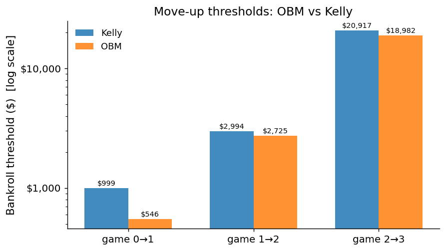
| Transition | Kelly threshold | OBM threshold | OBM / Kelly |
|---|---|---|---|
| Work → 1/2 | $999 | $546 | 0.55× |
| 1/2 → 2/5 | $2,994 | $2,725 | 0.91× |
| 2/5 → 5/10 | $20,917 | $18,982 | 0.91× |
OBM recommends moving up earlier at every transition. The gap is largest at the first step — the OBM threshold is 55% of Kelly’s — and narrows to around 9% at higher transitions.
The direction of this result is not obvious, because two forces act on the threshold in opposite directions. The first pushes the OBM threshold above Kelly: in this calibration, higher-stakes games have worse Sharpe ratios than lower-stakes games. In Kelly’s continuous world, risk and reward scale together linearly, so moving up is always proportionally attractive. With discrete games, the next game up may be a worse risk-adjusted bet per dollar of bankroll than the current one. This means the option value of moving up is lower than Kelly assumes, which, all else equal, would make the player less eager to reach the next threshold — implying a higher move-up bankroll, not a lower one.
Yet the net effect is a lower threshold. Some feature — or combination of features — of the discrete game structure dominates and pulls the threshold below Kelly’s. The recursive pricing of future optionality is the natural candidate: reaching the 1/2 game at a bankroll of $546 instead of $999 means getting to the 2/5 threshold sooner as well, which in turn means getting to 5/10 sooner. The OBM model prices the entire chain of future optionality; Kelly prices only today’s growth rate. This difference is largest at the first transition, where the full chain lies ahead, and smallest at the highest transition, where only one more step remains.
It is also consistent with the CRRA pattern from the finite-horizon model: at low bankrolls the recursive model is more risk-averse than Kelly (implying a higher threshold on risk-per-dollar grounds) and less risk-averse at high bankrolls (implying a lower threshold). The fact that the threshold ends up lower overall suggests the optionality-chain effect outweighs the risk-aversion effect in net. We do not decompose the two contributions further here, but the threshold ratios provide a clean reduced-form summary of their interaction.
4 Conclusion
Endogenous risk aversion. A risk-neutral player choosing among discrete games behaves as if risk-averse. The implied CRRA coefficient exceeds log utility (Kelly’s \(\eta = 1\)) at low bankrolls and falls below it at high bankrolls, declining toward zero once all move-up thresholds are behind the player. Kelly is a reasonable approximation in the middle of the bankroll distribution but underestimates risk aversion where it matters most — at low bankrolls, where the option value of the next game is largest relative to current stakes.
OBM vs Kelly thresholds. OBM recommends moving up at 55% of the Kelly threshold for the first transition and around 91% for subsequent transitions. Two opposing forces shape this result: worse Sharpe ratios at higher stakes push the threshold above Kelly, while recursive pricing of the full optionality chain pulls it below. The chain effect dominates, especially at the first transition where all future games lie ahead.
Tournament extensions. BRM considerations are likely most consequential in tournament poker, in two distinct ways. The first is game selection: choosing which tournaments to enter involves the same discrete-choice structure as cash game selection, but with higher variance and larger buyins relative to bankroll, amplifying the option-value effects documented here. The second is more subtle: BRM interacts with in-tournament decision making. Standard chip EV (CEV) analysis fails to account for ICM — the non-linear relationship between chips and prize equity. On top of this, both CEV and ICM ignore the risk aversion that arises from bankroll considerations. A player with a limited bankroll should be more risk-averse at the final table than either framework suggests, because chips represent not just prize equity but future playing capital.